41 how to add data labels to a 3d pie chart in excel

How to display leader lines in pie chart in Excel? - ExtendOffice To display leader lines in pie chart, you just need to check an option then drag the labels out. 1. Click at the chart, and right click to select Format Data Labels from context menu. 2. In the popping Format Data Labels dialog/pane, check Show Leader Lines in the Label Options section. See screenshot: Excel charts: add title, customize chart axis, legend and data labels ... Click anywhere within your Excel chart, then click the Chart Elements button and check the Axis Titles box. If you want to display the title only for one axis, either horizontal or vertical, click the arrow next to Axis Titles and clear one of the boxes: Click the axis title box on the chart, and type the text.

Pie Chart in Excel | How to Create Pie Chart - EDUCBA Step 1: Do not select the data; rather, place a cursor outside the data and insert one PIE CHART. Go to the Insert tab and click on a PIE. Step 2: once you click on a 2-D Pie chart, it will insert the blank chart as shown in the below image. Step 3: Right-click on the chart and choose Select Data.

How to add data labels to a 3d pie chart in excel

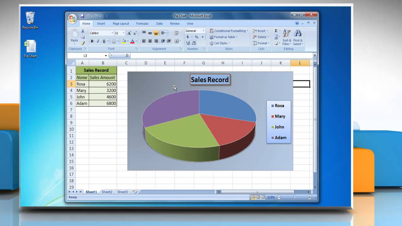
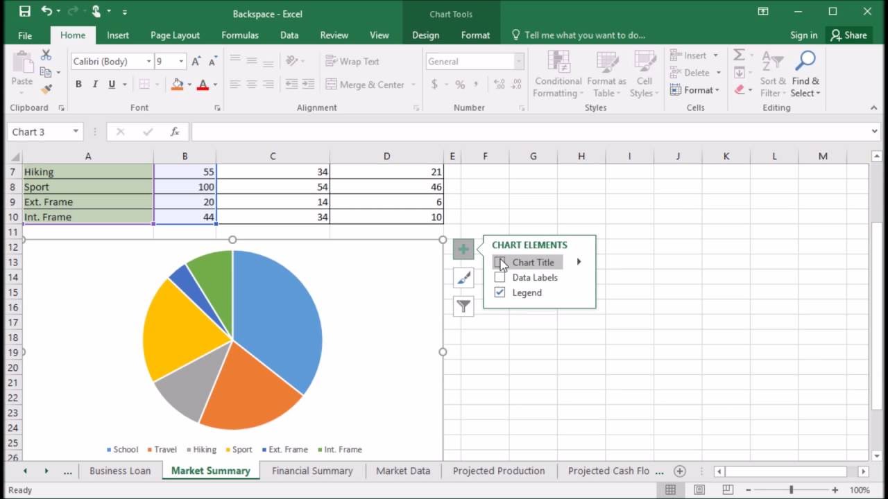
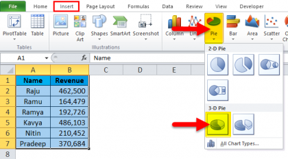
How to Create and Format a Pie Chart in Excel - Lifewire To create a pie chart, highlight the data in cells A3 to B6 and follow these directions: On the ribbon, go to the Insert tab. Select Insert Pie Chart to display the available pie chart types. Hover over a chart type to read a description of the chart and to preview the pie chart. Choose a chart type. Excel 3-D Pie charts - Microsoft Excel undefined 1. Select the data range (in this example, B3:C8 ). 2. On the Insert tab, in the Charts group, choose the Pie button: Choose the 3-D Pie chart. 3. Right-click in the chart area, then select Add Data Labels and click Add Data Labels in the popup menu: 4. Click in one of the labels to select all of them, then right-click and select Format Data ... Add a Data Callout Label to Charts in Excel 2013 - Software Tips and Tricks How to Add a Data Callout Label. Click on the data series or chart. In the upper right corner, next to your chart, click the Chart Elements button (plus sign), and then click Data Labels. A right pointing arrow will appear, click on this arrow to view the submenu. Select Data Callout.

How to add data labels to a 3d pie chart in excel. Excel 3-D Pie charts - Microsoft Excel 365 - OfficeToolTips 1. Select the data range (in this example, B3:C8 ). 2. On the Insert tab, in the Charts group, choose the Pie button: Choose the 3-D Pie chart. 3. Right-click in the chart area, then select Add Data Labels and click Add Data Labels in the popup menu: 4. Click in one of the labels to select all of them, then right-click and select Format Data ... Adding Data Labels to Your Chart (Microsoft Excel) - ExcelTips (ribbon) To add data labels in Excel 2013 or Excel 2016, follow these steps: Activate the chart by clicking on it, if necessary. Make sure the Design tab of the ribbon is displayed. (This will appear when the chart is selected.) Click the Add Chart Element drop-down list. Select the Data Labels tool. Inserting Data Label in the Color Legend of a pie chart Hi, I am trying to insert data labels (percentages) as part of the side colored legend, rather than on the pie chart itself, as displayed on the image ... There is no built-in way to do that, but you can use a trick: see Add Percent Values in Pie Chart Legend (Excel 2010) 0 Likes . Reply. Share. Share to LinkedIn; Share to Facebook; Share to ... How to Make a 3D Pie Chart in Excel? - GeeksforGeeks Step 2: Select all the elements of the table. Now, go to the Insert section. Locate Pie Charts under the Charts sub-section. The positioning of 'Pie Charts' may be different for different versions of Excel. Then, from the available 3D charts, select the one most suitable for your purpose of work. Now, wait for the Pie Chart to show up.

How to insert data labels to a Pie chart in Excel 2013 - YouTube This video will show you the simple steps to insert Data Labels in a pie chart in Microsoft® Excel 2013. Content in this video is provided on an "as is" basi... A Step-By-Step Guide on How to Make a Pie Chart in Excel 3. Select your data values and create the chart. Highlight the data range by clicking on the cell on the top left corner and dragging it until you've selected all the cells with values you wish to include in the pie chart. Then go to the top left corner of your window and click the "Insert" tab next to the "Home" tab. How to Create a Pie Chart in Excel - Smartsheet Enter data into Excel with the desired numerical values at the end of the list. Create a Pie of Pie chart. Double-click the primary chart to open the Format Data Series window. Click Options and adjust the value for Second plot contains the last to match the number of categories you want in the "other" category. Pie Charts in Excel - How to Make with Step by Step Examples Task b: Add data labels and data callouts. Step 3: Right-click the pie chart and expand the "add data labels" option. Next, choose "add data labels" again, as shown in the following image. Step 4: The data labels are added to the chart, as shown in the following image.

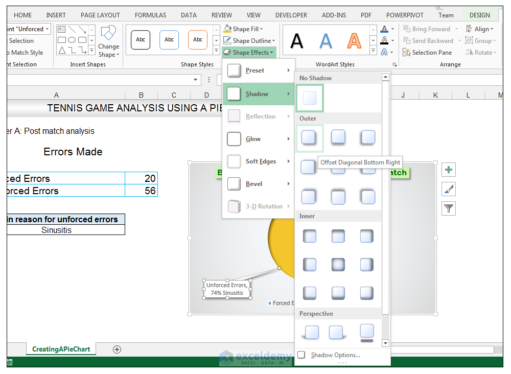
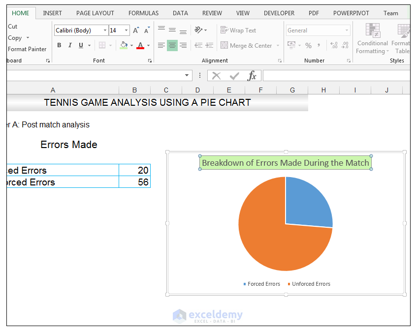
Add / Move Data Labels in Charts - Excel & Google Sheets Check Data Labels . Change Position of Data Labels. Click on the arrow next to Data Labels to change the position of where the labels are in relation to the bar chart. Final Graph with Data Labels. After moving the data labels to the Center in this example, the graph is able to give more information about each of the X Axis Series. Edit titles or data labels in a chart - support.microsoft.com To edit the contents of a title, click the chart or axis title that you want to change. To edit the contents of a data label, click two times on the data label that you want to change. The first click selects the data labels for the whole data series, and the second click selects the individual data label. Click again to place the title or data ... How to Create A 3-D Pie Chart in Excel [FREE TEMPLATE] The data in the table is pretty self-explanatory, so move on to the nitty-gritty. Here's the easiest way to create a 3-D pie chart: Select any cell in the data table ( A1:A6 ). Switch to the Insert tab. Choose " Insert Pie or Doughnut Chart. ". Click " 3-D Pie. ". Just a few clicks are your 3-D chart is ready to go: How to Make a Pie Chart in Excel & Add Rich Data Labels to The Chart! Creating and formatting the Pie Chart. 1) Select the data. 2) Go to Insert> Charts> click on the drop-down arrow next to Pie Chart and under 2-D Pie, select the Pie Chart, shown below. 3) Chang the chart title to Breakdown of Errors Made During the Match, by clicking on it and typing the new title. 4) With the chart title still selected, go to ...

Pie Chart in Excel | How to Create Pie Chart | Step-by-Step Guide Chart

2D & 3D Pie Chart in Excel - Tech Funda In last post, we learnt about creating Line chart in Excel.In this post, we shall learn how to create Pie chart, add filter and style to it. 2-D Pie Chart. To create 2-D Pie chart in Excel, first select the Chart data and go to INSERT menu and click on 'Insert Pie or Doughnut Chart' command dropdown under Charting group on the ribbon.. You will see a Pie chart appearing on the page as ...

How to Data Labels in a Pie chart in Excel 2007 - YouTube

Add or remove data labels in a chart - support.microsoft.com On the Design tab, in the Chart Layouts group, click Add Chart Element, choose Data Labels, and then click None. Click a data label one time to select all data labels in a data series or two times to select just one data label that you want to delete, and then press DELETE. Right-click a data label, and then click Delete.

How to Make Pie Chart in Microsoft Excel

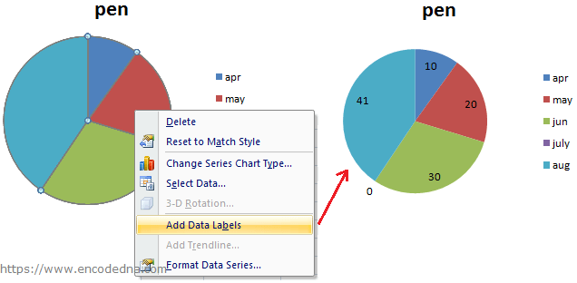
Possible to add second data label to pie chart? - Excel Help Forum Re: Possible to add second data label to pie chart? You get one data label per plotted point. I think you could use the. first trick in this page of Andy Pope's, and make the pie in front the. same size as the one in back, and use one pie for the outside labels and. the other for the inside labels.

Power BI Microsoft Dynamics CRM Online – PivotChart Report Part 2 - Microsoft Dynamics CRM Community

Excel 2010 data labels not showing on 3d pie chart If I then click on 'format data label' from the drop down list, and either select or de-select 'include legend key in label', the missing text appears on the other legends! Save the file, close it, re-open go back to the pie chart and the text is just on the one legend & missing from the others again! The graph also has data labels but they are ...

How to Make a PIE Chart in Excel (Easy Step-by-Step Guide)

How to Create Pie Charts in Excel (In Easy Steps) - Excel Easy Select the range A1:D1, hold down CTRL and select the range A3:D3. 6. Create the pie chart (repeat steps 2-3). 7. Click the legend at the bottom and press Delete. 8. Select the pie chart. 9. Click the + button on the right side of the chart and click the check box next to Data Labels.

How to Make a Pie Chart in Excel & Add Rich Data Labels to The Chart!

3D maps excel 2016 add data labels - Excel Help Forum Re: 3D maps excel 2016 add data labels. I don't think there are data labels equivalent to that in a standard chart. The bars do have a detailed tool tip but that required the map to be interactive and not a snapped picture. You could add annotation to each point. Select a stack and right click to Add annotation. Cheers.

406 How to remove chart title and add data labels to a Pie Chart in Excel 2016 - YouTube

Creating Pie Chart and Adding/Formatting Data Labels (Excel ... - YouTube Creating Pie Chart and Adding/Formatting Data Labels (Excel) Creating Pie Chart and Adding/Formatting Data Labels (Excel)

How to Make a Pie Chart in Excel & Add Rich Data Labels to The Chart!

How to show percentage in pie chart in Excel? - ExtendOffice Please do as follows to create a pie chart and show percentage in the pie slices. 1. Select the data you will create a pie chart based on, click Insert > I nsert Pie or Doughnut Chart > Pie. See screenshot: 2. Then a pie chart is created. Right click the pie chart and select Add Data Labels from the context menu. 3.

VBA Guide For Charts and Graphs - Automate Excel

Excel 3-D Pie charts - Microsoft Excel 2016 - OfficeToolTips If you want to create a pie chart that shows your company (in this example - Company A) in the greatest positive light: Do the following: 1. Select the data range (in this example, B5:C10 ). 2. On the Insert tab, in the Charts group, choose the Pie button: Choose 3-D Pie. 3. Right-click in the chart area, then select Add Data Labels and click ...

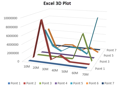
3D Plot in Excel | How to Plot 3D Graphs in Excel?

Microsoft Excel Tutorials: Add Data Labels to a Pie Chart - Home and Learn To add the numbers from our E column (the viewing figures), left click on the pie chart itself to select it: The chart is selected when you can see all those blue circles surrounding it. Now right click the chart. You should get the following menu: From the menu, select Add Data Labels. New data labels will then appear on your chart:

How to Create a Pie Chart in Excel using Worksheet Data

Add a Data Callout Label to Charts in Excel 2013 - Software Tips and Tricks How to Add a Data Callout Label. Click on the data series or chart. In the upper right corner, next to your chart, click the Chart Elements button (plus sign), and then click Data Labels. A right pointing arrow will appear, click on this arrow to view the submenu. Select Data Callout.

VBA Guide For Charts and Graphs - Automate Excel

Excel 3-D Pie charts - Microsoft Excel undefined 1. Select the data range (in this example, B3:C8 ). 2. On the Insert tab, in the Charts group, choose the Pie button: Choose the 3-D Pie chart. 3. Right-click in the chart area, then select Add Data Labels and click Add Data Labels in the popup menu: 4. Click in one of the labels to select all of them, then right-click and select Format Data ...

Pie Chart in Excel | How to Create Pie Chart | Step-by-Step Guide Chart

How to Create and Format a Pie Chart in Excel - Lifewire To create a pie chart, highlight the data in cells A3 to B6 and follow these directions: On the ribbon, go to the Insert tab. Select Insert Pie Chart to display the available pie chart types. Hover over a chart type to read a description of the chart and to preview the pie chart. Choose a chart type.

How to Create and Format a Pie Chart in Excel

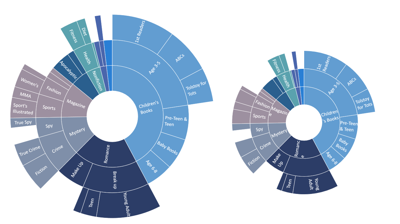
Breaking down hierarchical data with Treemap and Sunburst charts - Microsoft 365 Blog

Pie Chart in Excel | How to Create Pie Chart | Step-by-Step Guide Chart

ADMNEXC305308 Excel Training - How to Create a pie chart with data labels - Showezy Excel & Xero ...

Share :