43 pivot table concatenate row labels

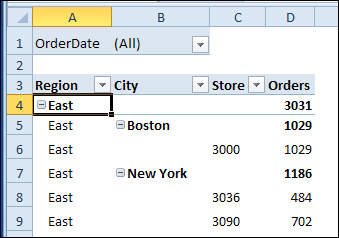
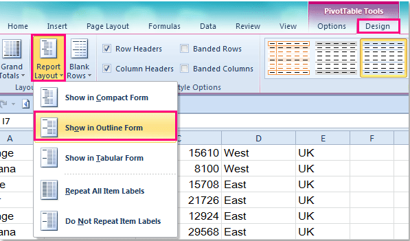
How to consolidate text with Pivot Table in Excel Right-click on the table name in the PivotTable Fields pane and click Add Measure. Give the measure a name and enter the formula based on your data. Then, click OK to add the measure. Once the measure is ready, move the category field ( Name) into Rows and new measure ( Abilities in our sample) into Values. The pivot table will show the results. How do I show multiple columns in a pivot table? Click any cell in your pivot table , and the PivotTable Tools tab will be displayed. Under the PivotTable Tools tab, click Design > Report Layout > Show in Tabular Form, see screenshot: And now, the row labels in the pivot table have been placed side by side at once, see screenshot: Excel Video 7 Multiple Rows and Columns in Pivot Tables

How To Change Column Names In A Pivot Table How To Change The Column Names Of Pivot Table In Google Sheets. Change Field Names In Pivot Table Source Data Excel Tables. Automatic Row And Column Pivot Table Labels. Change Field Names In Pivot Table Source Data Excel Tables. Centre Column Headings In Excel Pivot Table Tables. How To Rename Columns In Google Sheets 2 Methods Spreadsheet Point.

Pivot table concatenate row labels

Pivot table row labels side by side - Excel Tutorials You can copy the following table and paste it into your worksheet as Match Destination Formatting. Now, let's create a pivot table ( Insert >> Tables >> Pivot Table) and check all the values in Pivot Table Fields. Fields should look like this. Right-click inside a pivot table and choose PivotTable Options…. Check data as shown on the image below. Spreadsheets: Problems with Pivot Table Labels - CFO To return to a normal layout of the pivot table, follow these steps: 1. Select any cell inside the pivot table. The PivotTable Tools tabs appear in the Ribbon. 2. Go to Design tab of the ribbon. 3. From the Design tab, open the Report Layout dropdown. 4. Combining row labels in pivot table : excel - reddit As an example if the row labels are salesman and some of the cells from the raw table have James Bond and others have bond, or JB. Each of these iteration gets its own row in the pivot table. So my question is there a way to combine these rows manually. I'm hiding averages in the pivot table so I can't simply add then all. Thanks :)

Pivot table concatenate row labels. How to Concatenate Values of Pivot Table - Basic Excel Tutorial =CONCATENATE (C2, ", ", D2) Add a PivotTable with the combined address column Format the PivotTable to display the data in columns. Go to Pivot tools and click the design menu. On the layout group, choose report layout and select show in tabular form. The data will be displayed as shown below. Concatenate strings with a line break Design the layout and format of a PivotTable In the PivotTable, right-click the row or column label or the item in a label, point to Move, and then use one of the commands on the Move menu to move the item to another location. Select the row or column label item that you want to move, and then point to the bottom border of the cell. Group data in an Excel Pivot Table - Ablebits To group the data by date, right click on a date in a column or row of your PivotTable and choose Group. You can group by Seconds, Minutes, Hours, Days, Months, Quarters or Years and set the starting and ending times. For groupings like Year and Month the interval is set to 1, but for Days you can set your own interval so you can group at an ... How to make row labels on same line in pivot table? Make row labels on same line with PivotTable Options You can also go to the PivotTable Options dialog box to set an option to finish this operation. 1. Click any one cell in the pivot table, and right click to choose PivotTable Options, see screenshot: 2.

Pivot Table but Transpose values - Microsoft Tech Community Hi everyone, I am trying to figure out a formula/way to quickly transpose all city values from rows to columns for each ID number. As you can tell from below, some ID numbers have multiple cities listed whereas others only have 1-2. Regardless, I want the formula to look at each ID number, see ho... pivot table how to combine 2 row labels - MrExcel Message Board #1 Hi, i am having the pivot table in the below format. my concern is how i can combine both A & AA together the source is from data connection and not from the excel. This is pivot table output, my request is it possible to combine A & AA together in existing pivot table Look Like this: Thanks in advance, SK Concatenate Unique Text Values in an Excel Pivot Table In this video we're going to learn how to concatenate the unique values from our data and show them inside an Excel pivot table.Link to previous video on sum... 5 Ways to Concatenate Data with a Line Break in Excel This will allow us to create measures using the DAX fomula language within out pivot tables. In the PivotTable Fields window, right click on the table name and choose Add Measure. =CONCATENATEX ('ContactList','ContactList' [Address]," ") Add a Measure Name like Label,then enter the above formula for the measure and press the OK button.

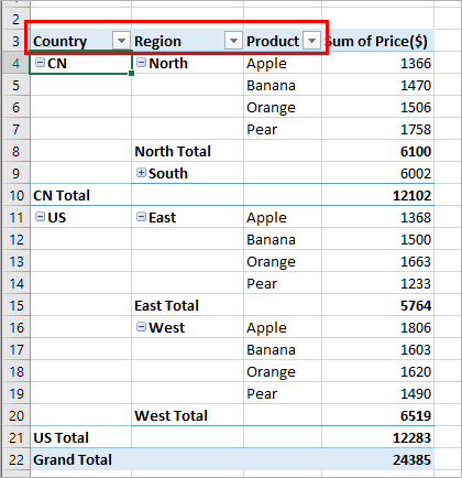
Combining two+ Columns to form one Row label column in Pivot Table Re: Combining two+ Columns to form one Row label column in Pivot Table Select a cell in your pivot table. Press Alt, then D, then P (i.e. in succession; not all at the same time), to call up the Pivot Table Wizard. Click "" button twice. Combining two date fields into one PivotTable Row Label You will have to first rearrange your source data into a 3 column using Power Query a.k.a. Get & Transform in Excel 2016. Once done, you can easily create your desired Pivot Table. To rearrange the dataset, use the "Unpivot other columns" feature of Power Query. Here's a screenshot. Regards, Ashish Mathur Pivot table row labels in separate columns • AuditExcel.co.za So when you click in the Pivot Table and click on the DESIGN tab one of the options is the Report Layout. Click on this and change it to Tabular form. Your pivot table report will now look like the bottom picture and will be easier to use in other areas of the spreadsheet and in our opinion is also easier to read. Who wants to be a ... How to rename group or row labels in Excel PivotTable? 1. Click at the PivotTable, then click Analyze tab and go to the Active Field textbox. 2. Now in the Active Field textbox, the active field name is displayed, you can change it in the textbox. You can change other Row Labels name by clicking the relative fields in the PivotTable, then rename it in the Active Field textbox.

Repeat Pivot Table row labels • AuditExcel.co.za Pivot Tables Course

Concatenate rows values - Microsoft Power BI Community Solved: Hi everyone, I have a table in a databse which has job numbers, template nuber, and comments. I have managed to do a bunch or merges, pivots, ... Concatenate rows values ‎06-09-2016 11:52 PM. Hi everyone, ... Labels: Labels: Need Help; Message 1 of 3 36,799 Views 0 Reply. 1 ACCEPTED SOLUTION

How to Sort Pivot Table Row Labels, Column Field Labels and Data Values with Excel VBA Macro ...

How To Compare Multiple Lists of Names with a Pivot Table Step #2 - Create the Pivot Table. We can now create a Pivot Table based on our 'Combined Data' list to start making comparisons. Here are the steps to creating the Pivot Table. Select a cell in the Combined List and press the Pivot Table button on the Insert tab of the Ribbon.

How to Sort Pivot Table Row Labels, Column Field Labels and Data Values with Excel VBA Macro ...

3 Ways to Display (Multiple Items) Filter Criteria in a Pivot Table The quickest way to see a list of the Multiple Items in the filter is to add a slicer to the pivot table. Select any cell in the pivot table. Select the Analyze/Options tab in the ribbon. Click the Insert Slicer button. Check the box for the field that is in the Filters area with the filter applied to it. Press OK.

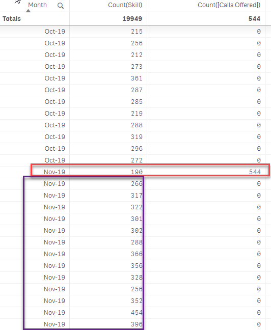
How to sum up the count measure by month and year ... - Qlik Community - 1661550

merge - Excel Pivot Table - Combine rows - Stack Overflow 1 Follow the steps - 1. Right click on any one of the dates in column 1 (dates & time). 2. Select "Group..." in the dropdown. 3. In the pop-up select "By" >>> "Days" 4. Select the "Number of days" range, in your case it would be 1. 5. Click OK. Hopefully you'll get your desired result. Share answered Sep 21, 2018 at 11:02 Nikzad Shahmardani 11 3

Excel Pivot Table Combine Columns | Decoration Items Image

How to Use Excel Pivot Table Label Filters Watch the steps in this short video, and the written instructions are below the video. Play. To change the Pivot Table option to allow multiple filters: Right-click a cell in the pivot table, and click PivotTable Options. Click the Totals & Filters tab Under Filters, add a check mark to 'Allow multiple filters per field.'.

30 Pivot Table Blank Row Label - Labels Database 2020

Repeat item labels in a PivotTable - support.microsoft.com Right-click the row or column label you want to repeat, and click Field Settings. Click the Layout & Print tab, and check the Repeat item labels box. Make sure Show item labels in tabular form is selected. Notes: When you edit any of the repeated labels, the changes you make are applied to all other cells with the same label.

Accelerate Your Analysis with Pivot Table | Simplified Excel

Grouping labels and concatenating their text values (like a pivot table) Then concatenate a comma with each of your transposed attributes in a final results column. Admittedly all this "copy/paste special/transpose" would get old quickly if you have a long list of Products. If you have lots of data, using a few formulas you can work your way to the final result, as shown below.

Insert Blank Rows In a Pivot Table - Free Microsoft Excel Tutorials

How to Customize Your Excel Pivot Chart Data Labels - dummies The Data Labels command on the Design tab's Add Chart Element menu in Excel allows you to label data markers with values from your pivot table. When you click the command button, Excel displays a menu with commands corresponding to locations for the data labels: None, Center, Left, Right, Above, and Below. None signifies that no data labels ...

Pivot table row labels in separate columns • AuditExcel.co.za

Combining row labels in pivot table : excel - reddit As an example if the row labels are salesman and some of the cells from the raw table have James Bond and others have bond, or JB. Each of these iteration gets its own row in the pivot table. So my question is there a way to combine these rows manually. I'm hiding averages in the pivot table so I can't simply add then all. Thanks :)

Importing a Hierarchy Tree Structure | Monarch Tracking

Spreadsheets: Problems with Pivot Table Labels - CFO To return to a normal layout of the pivot table, follow these steps: 1. Select any cell inside the pivot table. The PivotTable Tools tabs appear in the Ribbon. 2. Go to Design tab of the ribbon. 3. From the Design tab, open the Report Layout dropdown. 4.