44 excel pie chart with lines to labels

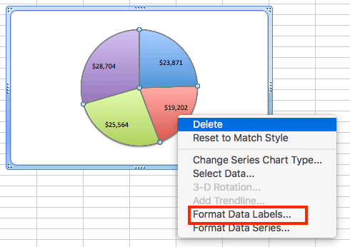
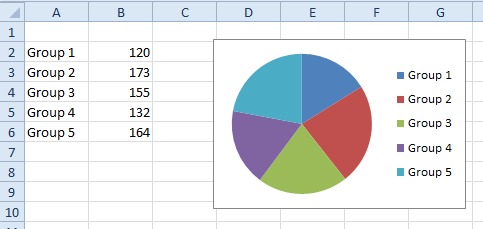
How to fix wrapped data labels in a pie chart - Sage Intelligence 1. Right click on the data label and select Format Data Labels. 2. Select Text Options > Text Box > and un-select Wrap text in shape. 3. The data labels resize to fit all the text on one line. 4. Alternatively, by double-clicking a data label, the handles can be used to resize the label to wrap words as desired. How to Create Pie Charts in Excel (In Easy Steps) 1. Select the range A1:D2. 2. On the Insert tab, in the Charts group, click the Pie symbol. 3. Click Pie. Result: 4. Click on the pie to select the whole pie. Click on a slice to drag it away from the center. Result: Note: only if you have numeric labels, empty cell A1 before you create the pie chart.

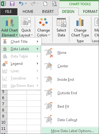
Change the format of data labels in a chart To get there, after adding your data labels, select the data label to format, and then click Chart Elements > Data Labels > More Options. To go to the appropriate area, click one of the four icons ( Fill & Line, Effects, Size & Properties ( Layout & Properties in Outlook or Word), or Label Options) shown here.

Excel pie chart with lines to labels

Creating Pie Chart and Adding/Formatting Data Labels (Excel) Creating Pie Chart and Adding/Formatting Data Labels (Excel) How to add Axis Labels (X & Y) in Excel & Google Sheets Edit Chart Axis Labels. Click the Axis Title; Highlight the old axis labels; Type in your new axis name; Make sure the Axis Labels are clear, concise, and easy to understand. Dynamic Axis Titles. To make your Axis titles dynamic, enter a formula for your chart title. Click on the Axis Title you want to change Excel Doughnut chart with leader lines - teylyn Step 2 - add the same data series as a pie chart Step 3 - Add data labels for the pie chart Select the pie chart and add data labels. They will be positioned outside of the pie. Click each data label and drag it a bit to see the leader lines appear. Step 3 - Add data labels for the pie chart Step 4 - Hide the pie chart

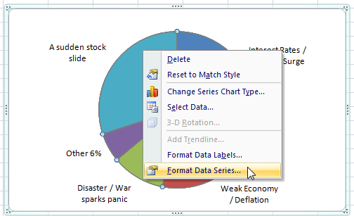
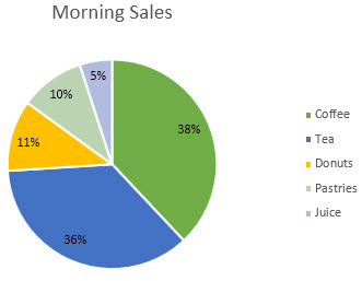
Excel pie chart with lines to labels. How to make a pie chart in Excel - Ablebits To rotate a pie chart in Excel, do the following: Right-click any slice of your pie graph and click Format Data Series. On the Format Data Point pane, under Series Options, drag the Angle of first slice slider away from zero to rotate the pie clockwise. Or, type the number you want directly in the box. Pie Chart in Excel | How to Create Pie Chart - EDUCBA Step 1: Select the data to go to Insert, click on PIE, and select 3-D pie chart. Step 2: Now, it instantly creates the 3-D pie chart for you. Step 3: Right-click on the pie and select Add Data Labels. This will add all the values we are showing on the slices of the pie. Add / Move Data Labels in Charts - Excel & Google Sheets Add and Move Data Labels in Google Sheets. Double Click Chart. Select Customize under Chart Editor. Select Series. 4. Check Data Labels. 5. Select which Position to move the data labels in comparison to the bars. How to Create and Format a Pie Chart in Excel - Lifewire To add data labels to a pie chart: Select the plot area of the pie chart. Right-click the chart. Select Add Data Labels . Select Add Data Labels. In this example, the sales for each cookie is added to the slices of the pie chart. Change Colors

Leader lines for Pie chart are appearing only when the data labels are ... Mar 2, 2017. #2. Leader lines are deemed not necessary in the default position (e.g., outside end). It's only when they are moved, the leader lines are possibly needed because they are further from the point they are labeling. Best fit tries (as best Excel can) to arrange the labels without overlapping. It the wedges are large enough, the ... How to Create Line Charts in Excel (In Easy Steps) Use a scatter plot (XY chart) to show scientific XY data. To create a line chart, execute the following steps. 1. Select the range A1:D7. 2. On the Insert tab, in the Charts group, click the Line symbol. 3. Click Line with Markers. Note: only if you have numeric labels, empty cell A1 before you create the line chart. How to add leader lines to doughnut chart in Excel? Select data and click Insert > Other Charts > Doughnut. In Excel 2013, click Insert > Insert Pie or Doughnut Chart > Doughnut. 2. Select your original data again, and copy it by pressing Ctrl + C simultaneously, and then click at the inserted doughnut chart, then go to click Home > Paste > Paste Special. See screenshot: 3. Excel Pie Chart Line To Labels Details: To display leader lines in pie chart, you just need to check an option then drag the labels out. 1. Click at the chart, and right click to select Format Data Labels from context menu. 2. In the popping Format Data Labels dialog/pane, check … excel create pie chart from list › Verified 3 days ago › Url: extendoffice.com Go Now

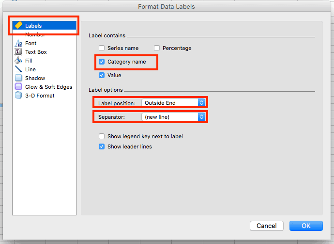
Pie Chart in Excel - Inserting, Formatting, Filters, Data Labels Right click on the Data Labels on the chart. Click on Format Data Labels option. Consequently, this will open up the Format Data Labels pane on the right of the excel worksheet. Mark the Category Name, Percentage and Legend Key. Also mark the labels position at Outside End. This is how the chark looks. Formatting the Chart Background, Chart Styles How to display leader lines in pie chart in Excel? To display leader lines in pie chart, you just need to check an option then drag the labels out. 1. Click at the chart, and right click to select Format Data Labels from context menu. 2. In the popping Format Data Labels dialog/pane, check Show Leader Lines in the Label Options section. See screenshot: 3. Excel custom pie chart labels - Microsoft Community Excel custom pie chart labels. I want to use a pivot table to make a pie chart out of this. I want each of the pieces of the pie to contain the number of entries and between parentheses the percentage. So in the "Yes" piece, there should be '3 (33%)'. Actually, if I hover the pie chart in Excel, I get exactly the notation O want! pie chart with data labels [SOLVED] - Excel Help Forum In the "Format Data Labels" popup: Label Options: Label Contains: Check "Category Name", "Value", and "Percentage". Label Position: "Inside End" Radio Button (already selected in your posted chart) At the bottom, change "Separator" to " (New Line)" That should do what you want. Register To Reply.

33 How To Label Pie Chart In Excel - Labels Design Ideas 2020

How to Create a Pie Chart in Excel | Smartsheet Enter data into Excel with the desired numerical values at the end of the list. Create a Pie of Pie chart. Double-click the primary chart to open the Format Data Series window. Click Options and adjust the value for Second plot contains the last to match the number of categories you want in the "other" category.

Excel Charts: Excel Pie Chart With Individual Slice Radius

Excel Pie Chart Lines to Labels, in Access Report If I put an Excel 2010 2-D pie chart into an Access 2010 report, and have a data label for each part of the pie, with lines from the data labels to the parts of the pie, and then size the chart, the lines are OK in edit mode, but become much heavier when in design mode or when viewing or printing the chart.

Tip : HTML-5 Pie chart long label wrapping in Jasper Studio 6.x & Jasper Server 6.x (OR ...

Dynamically Label Excel Chart Series Lines - My Online Training Hub Select the outer edge of the chart to expose the contextual Chart Tools ribbon tabs Select the Format tab (In Excel 2007 & 2010 it's the Layout tab) Click on the drop down Select the first label series: Step 4: Add the Labels Excel 2013/2016 Click the + icon beside the chart as shown below (Note: for Excel 2007/2010 go to Layout tab) Data Labels

How to Create Excel Pie Charts & Add Rich Data Labels to The Chart!

Add or remove data labels in a chart - support.microsoft.com In the upper right corner, next to the chart, click Add Chart Element > Data Labels. To change the location, click the arrow, and choose an option. If you want to show your data label inside a text bubble shape, click Data Callout. To make data labels easier to read, you can move them inside the data points or even outside of the chart.

SQL & BI Learning: Pie Chart with data labels outside in ssrs

How-to Add Label Leader Lines to an Excel Pie Chart - YouTube Step-by-Step Tutorial: how-to create label leader lines that connect pie labels that are outsi...

How to make a Pie Chart in Microsoft Excel | hubpages

How to Make a 2010 Excel Pie Chart with Labels Both Inside and Outside Harassment is any behavior intended to disturb or upset a person or group of people. Threats include any threat of suicide, violence, or harm to another.

How-to Make a WSJ Excel Pie Chart with Labels Both Inside and Outside - Excel Dashboard Templates

Excel charts: add title, customize chart axis, legend and data labels ... Click anywhere within your Excel chart, then click the Chart Elements button and check the Axis Titles box. If you want to display the title only for one axis, either horizontal or vertical, click the arrow next to Axis Titles and clear one of the boxes: Click the axis title box on the chart, and type the text.

Add data labels to a chart - Office Support

Directly Labeling in Excel - Evergreen Data If it pops in your value instead of the name of your series, right-click on it again and select Format Data Label (WATCH FOR THE PLURAL/SINGULAR BUSINESS HERE). In the dialogue box that opens, check Series and uncheck Value. Boom. Way #2 Insert a text box at the end of the line and type the label name. You know how to insert a text box, right?

How to Create a Pie Chart in Excel | Smartsheet

Excel Doughnut chart with leader lines - teylyn Step 2 - add the same data series as a pie chart Step 3 - Add data labels for the pie chart Select the pie chart and add data labels. They will be positioned outside of the pie. Click each data label and drag it a bit to see the leader lines appear. Step 3 - Add data labels for the pie chart Step 4 - Hide the pie chart

Insert a pie chart in Excel - Excel

How to add Axis Labels (X & Y) in Excel & Google Sheets Edit Chart Axis Labels. Click the Axis Title; Highlight the old axis labels; Type in your new axis name; Make sure the Axis Labels are clear, concise, and easy to understand. Dynamic Axis Titles. To make your Axis titles dynamic, enter a formula for your chart title. Click on the Axis Title you want to change