41 excel add data labels to all series
Excel 2010: How to format ALL data point labels SIMULTANEOUSLY Click here to reveal answer 1 2 3 Next G gehusi Board Regular Joined Jul 20, 2010 Messages 182 May 24, 2011 #2 Instead of selecting the entire chart, right click one of the data points and select "Format Data Labels". B brianclong Board Regular Joined Apr 11, 2006 Messages 168 May 24, 2011 #3 This still only formats one set of data series labels. Change the format of data labels in a chart To get there, after adding your data labels, select the data label to format, and then click Chart Elements > Data Labels > More Options. To go to the appropriate area, click one of the four icons ( Fill & Line, Effects, Size & Properties ( Layout & Properties in Outlook or Word), or Label Options) shown here.
How to set all data labels with Series Name at once in an Excel 2010 ... chart series data labels are set one series at a time. If you don't want to do it manually, you can use VBA. Something along the lines of. Sub setDataLabels () '. ' sets data labels in all charts. '. Dim sr As Series. Dim cht As ChartObject.

Excel add data labels to all series
How To Add Data Labels In Excel - veganheath.info To get there, after adding your data labels, select the data label to format, and then click chart elements > data labels > more options. After picking the series, click the data point you want to label. Source: temotips.blogspot.com. Using excel chart element button to add axis labels. Click the chart to show the chart elements button. Series.DataLabels method (Excel) | Microsoft Learn This example sets the data labels for series one on Chart1 to show their key, assuming that their values are visible when the example runs. With Charts("Chart1").SeriesCollection(1) .HasDataLabels = True With .DataLabels .ShowLegendKey = True .Type = xlValue End With End With. Support and feedback. chandoo.org › wp › change-data-labels-in-chartsHow to Change Excel Chart Data Labels to Custom Values? May 05, 2010 · First add data labels to the chart (Layout Ribbon > Data Labels) Define the new data label values in a bunch of cells, like this: Now, click on any data label. This will select “all” data labels. Now click once again. At this point excel will select only one data label.
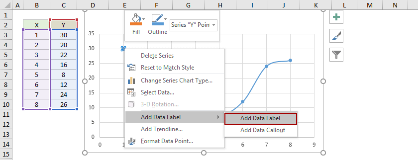
Excel add data labels to all series. how to add data labels into Excel graphs - storytelling with data You can download the corresponding Excel file to follow along with these steps: Right-click on a point and choose Add Data Label. You can choose any point to add a label—I'm strategically choosing the endpoint because that's where a label would best align with my design. Excel defaults to labeling the numeric value, as shown below. Add a DATA LABEL to ONE POINT on a chart in Excel Method — add one data label to a chart line Steps shown in the video above: Click on the chart line to add the data point to. All the data points will be highlighted. Click again on the single point that you want to add a data label to. Right-click and select 'Add data label' This is the key step! Create Dynamic Chart Data Labels with Slicers - Excel Campus Step 6: Setup the Pivot Table and Slicer. The final step is to make the data labels interactive. We do this with a pivot table and slicer. The source data for the pivot table is the Table on the left side in the image below. This table contains the three options for the different data labels. support.microsoft.com › en-us › officeAdd or remove data labels in a chart - support.microsoft.com Depending on what you want to highlight on a chart, you can add labels to one series, all the series (the whole chart), or one data point. Add data labels. You can add data labels to show the data point values from the Excel sheet in the chart. This step applies to Word for Mac only: On the View menu, click Print Layout.
How to Fix Data Model Relationships Not Working in Excel To manually create a data model relationship in Excel, follow the steps discussed below: 1. Firstly, we need to open the PivotTable Fields. So right-click on the table and select Show Field List. 2. Secondly, the PivotTable Fields will appear on the right side. From there, select the All tab. How To Create Labels In Excel - bernd-abel.info Column names in your spreadsheet match the field names you want to insert in your labels. Right click the data series in the chart, and select add data labels > add data labels from the context menu to add data labels. In the mailings tab of word, select the finish & merge option and choose edit individual documents from the menu. How to Add Labels to Scatterplot Points in Excel - Statology Step 3: Add Labels to Points. Next, click anywhere on the chart until a green plus (+) sign appears in the top right corner. Then click Data Labels, then click More Options…. In the Format Data Labels window that appears on the right of the screen, uncheck the box next to Y Value and check the box next to Value From Cells. Changing data label format for all series in a pivot chart To change data labels format, please perform the following steps: Click the pivot chart > + sign near tthe pivot chart > right click data label of any series > Format Data Series... Besides, to move forward, could you please provide the following information? 1. Do all series have data labels when you create a pivot chart?
› dynamically-labelDynamically Label Excel Chart Series Lines • My Online ... Dynamically Label Excel Chart Series Lines Step 1: Duplicate the Series. Select columns B:J and insert a line chart (do not include column A). To modify the axis... Step 2: Clever Formula. The Label Series Data contains a formula that only returns the value for the last row of data. . Step 3: ... Adding Data Labels to a Chart Using VBA Loops - Wise Owl To do this, add the following line to your code: 'make sure data labels are turned on FilmDataSeries.HasDataLabels = True This simple bit of code uses the variable we set earlier to turn on the data labels for the chart. Without this line, when we try to set the text of the first data label our code would fall over. Excel chart changing all data labels from value to series name ... My graph has multiple columns and hundreds of stacked values (series) in each column. By selecting chart then from layout->data labels->more data labels options ->label options ->label contains-> (select)series name, I can only get one series name replacing its respective label values. Excel Charts: Dynamic Label positioning of line series - XelPlus Select your chart and go to the Format tab, click on the drop-down menu at the upper left-hand portion and select Series "Budget". Go to Layout tab, select Data Labels > Right. Right mouse click on the data label displayed on the chart. Select Format Data Labels. Under the Label Options, show the Series Name and untick the Value.
Adding rich data labels to charts in Excel 2013 | Microsoft ...
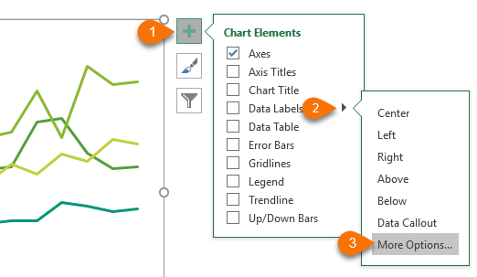
Adding Data Labels to Your Chart (Microsoft Excel) - ExcelTips (ribbon) Select the position that best fits where you want your labels to appear. To add data labels in Excel 2013 or later versions, follow these steps: Activate the chart by clicking on it, if necessary. Make sure the Design tab of the ribbon is displayed. (This will appear when the chart is selected.) Click the Add Chart Element drop-down list.

How to add live total labels to graphs and charts in Excel ...
Excel tutorial: How to use data labels When you check the box, you'll see data labels appear in the chart. If you have more than one data series, you can select a series first, then turn on data labels for that series only. You can even select a single bar, and show just one data label. In a bar or column chart, data labels will first appear outside the bar end.
How to Create a Graph with Multiple Lines in Excel | Pryor ...
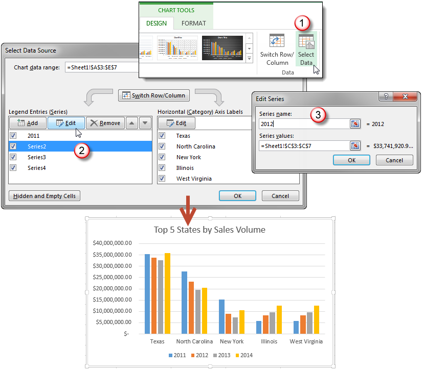
support.microsoft.com › en-us › officeAdd a data series to your chart - support.microsoft.com Leaving the dialog box open, click in the worksheet, and then click and drag to select all the data you want to use for the chart, including the new data series. The new data series appears under Legend Entries (Series) in the Select Data Source dialog box.

How to add data labels from different column in an Excel chart?
How to add or move data labels in Excel chart? - ExtendOffice In Excel 2013 or 2016. 1. Click the chart to show the Chart Elements button . 2. Then click the Chart Elements, and check Data Labels, then you can click the arrow to choose an option about the data labels in the sub menu. See screenshot: In Excel 2010 or 2007. 1. click on the chart to show the Layout tab in the Chart Tools group. See screenshot: 2.

Excel Charts: Dynamic Label positioning of line series
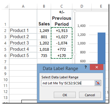
How to Use Cell Values for Excel Chart Labels - How-To Geek Select the chart, choose the "Chart Elements" option, click the "Data Labels" arrow, and then "More Options." Uncheck the "Value" box and check the "Value From Cells" box. Select cells C2:C6 to use for the data label range and then click the "OK" button. The values from these cells are now used for the chart data labels.

How to add or move data labels in Excel chart?
How to Add Data Labels to an Excel 2010 Chart - dummies Use the following steps to add data labels to series in a chart: Click anywhere on the chart that you want to modify. On the Chart Tools Layout tab, click the Data Labels button in the Labels group. None: The default choice; it means you don't want to display data labels. Center to position the data labels in the middle of each data point.
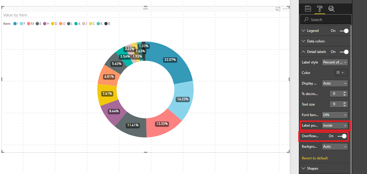
Solved: How to show all detailed data labels of pie chart ...
vba code to all datallabels on all series in a chart sub apply_data_labels () 'applies data labels to all 'data series on the set chart 'set number format of data labels const numformat = " [$$-409]#,##0.00_ ; [red]- [$$-409]#,##0.00 " dim cht as chart dim ser as series 'set the chart set cht = activesheet.chartobjects ("chart 1").chart 'apply data lables for each ser in …

How to Make Pie Chart with Labels both Inside and Outside ...
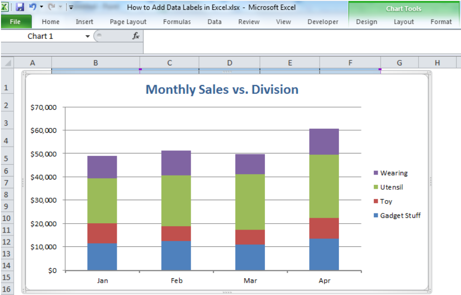
How to Add Labels to Show Totals in Stacked Column Charts in Excel In the chart, right-click the "Total" series and then, on the shortcut menu, select Add Data Labels. 9. Next, select the labels and then, in the Format Data Labels pane, under Label Options, set the Label Position to Above. 10. While the labels are still selected set their font to Bold. 11.
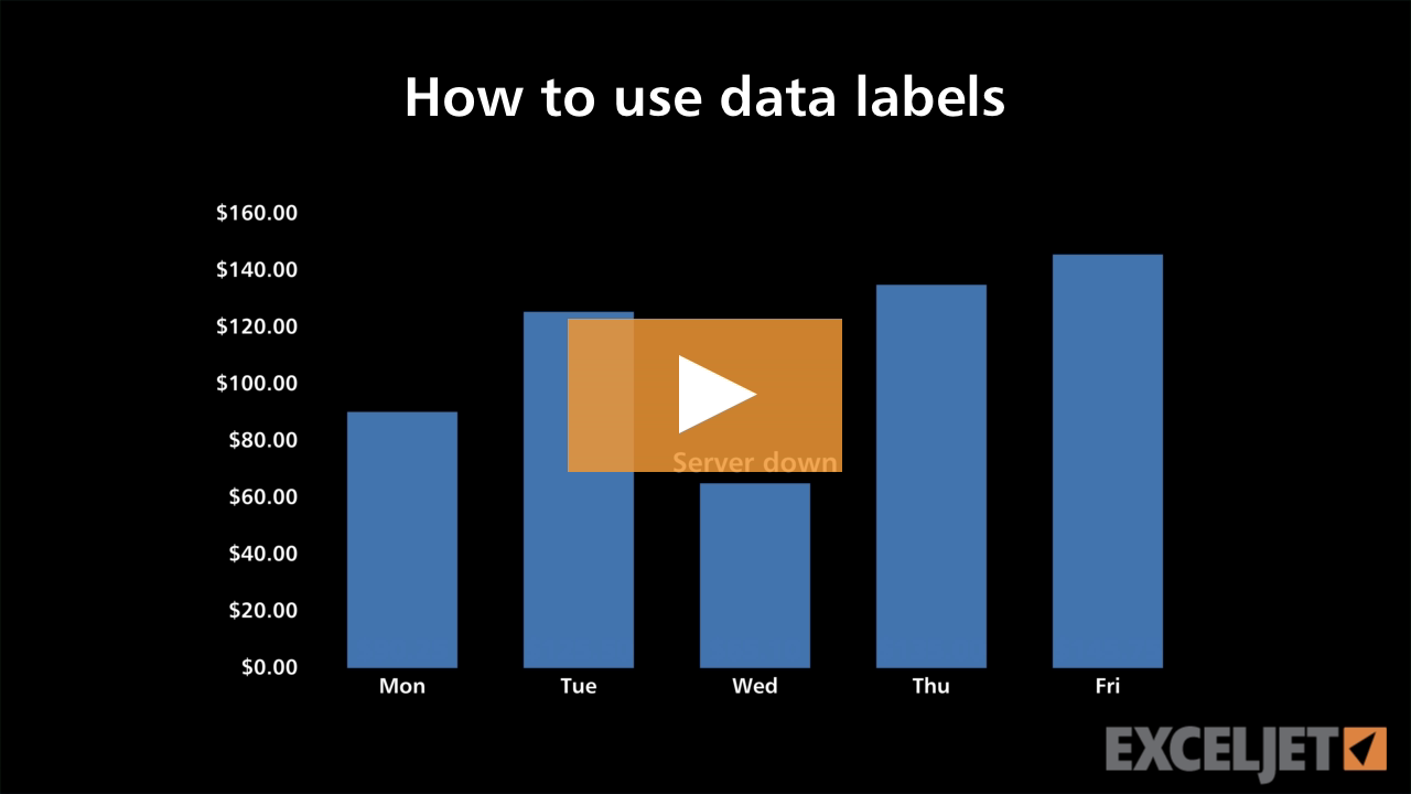
Excel tutorial: How to use data labels
› excel › how-to-add-total-dataHow to Add Total Data Labels to the Excel Stacked Bar Chart The basic chart function does not allow you to add a total data label that accounts for the sum of the individual components. Fortunately, creating these labels manually is a fairly simply process. Step 1: Create a sum of your stacked components and add it as an additional data series (this will distort your graph initially)

How to Add and Remove Chart Elements in Excel
› 682077 › how-to-rename-a-dataHow to Rename a Data Series in Microsoft Excel - How-To Geek Jul 27, 2020 · A data series in Microsoft Excel is a set of data, shown in a row or a column, which is presented using a graph or chart. To help analyze your data, you might prefer to rename your data series. Rather than renaming the individual column or row labels, you can rename a data series in Excel by editing the graph or chart.

Display Customized Data Labels on Charts & Graphs
Create A Pie Chart In Excel With and Easy Step-By-Step Guide Once you have all your data in place, follow these steps to create a pie chart: Step 1: Select the whole dataset. Step 2: Click on the Insert tab. Step 3: Now, in the charts group, you need to click on the "Insert Pie or Doughnut Chart" option. Step 4: Click on the pie icon that is within the 2-D pie icons.

Adding rich data labels to charts in Excel 2013 | Microsoft ...
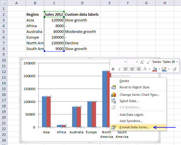
› documents › excelHow to add data labels from different column in an Excel chart? This method will guide you to manually add a data label from a cell of different column at a time in an Excel chart. 1. Right click the data series in the chart, and select Add Data Labels > Add Data Labels from the context menu to add data labels. 2. Click any data label to select all data labels, and then click the specified data label to select it only in the chart.

microsoft excel - Adding data label only to the last value ...
Formatting ALL data labels for ALL data series at once Jan 17, 2008. #2. You can pick Show Series for all series of labels at once, if you select the. chart, go to the Chart menu > Chart Options > Data Labels tab. This does all. series at once, not just the ones you've already labeled. You cannot apply other formatting to more than one series of labels at a. time. - Jon.

Enable or Disable Excel Data Labels at the click of a button ...
chandoo.org › wp › change-data-labels-in-chartsHow to Change Excel Chart Data Labels to Custom Values? May 05, 2010 · First add data labels to the chart (Layout Ribbon > Data Labels) Define the new data label values in a bunch of cells, like this: Now, click on any data label. This will select “all” data labels. Now click once again. At this point excel will select only one data label.
/simplexct/BlogPic-h7046.jpg)
How to Create a Bar Chart With Labels Above Bars in Excel
Series.DataLabels method (Excel) | Microsoft Learn This example sets the data labels for series one on Chart1 to show their key, assuming that their values are visible when the example runs. With Charts("Chart1").SeriesCollection(1) .HasDataLabels = True With .DataLabels .ShowLegendKey = True .Type = xlValue End With End With. Support and feedback.

Google Workspace Updates: Get more control over chart data ...
How To Add Data Labels In Excel - veganheath.info To get there, after adding your data labels, select the data label to format, and then click chart elements > data labels > more options. After picking the series, click the data point you want to label. Source: temotips.blogspot.com. Using excel chart element button to add axis labels. Click the chart to show the chart elements button.

Excel charts: add title, customize chart axis, legend and ...

How to set all data labels with Series Name at once in an ...
Custom data labels in a chart
Dynamically Label Excel Chart Series Lines • My Online ...

Dynamically Label Excel Chart Series Lines • My Online ...
How-to Use Data Labels from a Range in an Excel Chart - Excel ...

microsoft excel - Adding data label only to the last value ...

excel - How to show series-Legend label name in data labels ...

Chart Data Labels in PowerPoint 2013 for Windows

How To Show Or Hide Data Labels On MS Excel? | My Windows Hub

Quick Tip: Excel 2013 offers flexible data labels | TechRepublic

Apply Custom Data Labels to Charted Points - Peltier Tech
How to add data labels from different column in an Excel chart?
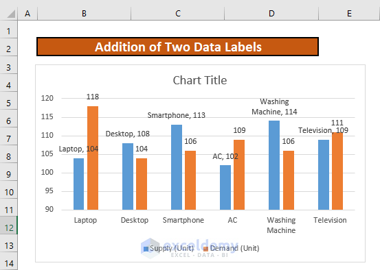
How to Add Two Data Labels in Excel Chart (with Easy Steps ...

How to Add Data Labels to an Excel 2010 Chart - dummies

How to Place Labels Directly Through Your Line Graph in ...

How to Add Total Data Labels to the Excel Stacked Bar Chart ...
How to Add Data Labels in Excel - Excelchat | Excelchat
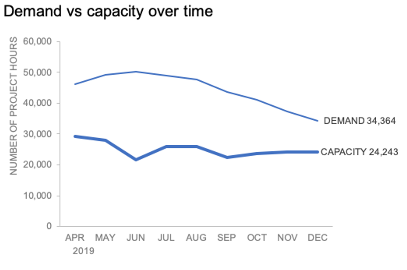
how to add data labels into Excel graphs — storytelling with data

Add or remove data labels in a chart

How to add data labels from different column in an Excel chart?

How to Add Data Labels to your Excel Chart in Excel 2013
About Data Labels

how to add data labels into Excel graphs — storytelling with data

Add or remove data labels in a chart
Post a Comment for "41 excel add data labels to all series"